About - Publications - Blog

Maximizing the Power Gains

Types of power gain

If you haven't read the definitions of the most commonly used power gains, you should probably do this first. We first briefly recap before maximizing the gains.

Consider a network "Z" with one input and one output (a two-port network). The input is connected to a generator (a voltage source V_G with internal impedance Z_G) and the output to a load impedance Z_L.

• We call the input impedance of the network Z_in=R_in+j.X_in. Note that the input impedance Z_inis dependent on Z_L (see figure).
• We call the output impedance Z_out=R_out+j.X_out. Note that the output impedance Z_inis dependent on Z_G (see figure).

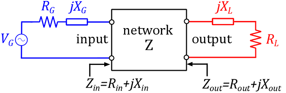
Figure 1: A network Z is connected to a generator at the input, and a load at the output

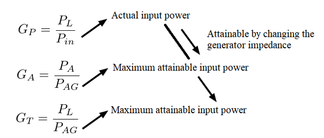
The operating power gain G_P

The operating power gain G_P is defined as the ratio of the power dissipated in the load Z_L to the power that the generator delivers to the network Z, connected to that load Z_L:

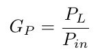
The gain depends on the network Z and on the load value Z_L, but is independent on Z_G. This power gain is sometimes called 'the efficiency' of the system.

Available gain G_A

The available gain G_A is defined as the ratio of the maximum available load power P_A to the available input power P_AG :

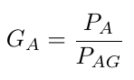
The available gain G_A is independent on Z_L. The gain depends on the network Z and on the generator impedance value Z_G.

Transducer gain G_T

The transducer gain G_T is defined as the ratio of the power dissipated in the load Z_L to the available input power P_AG of the generator:

It is dependent on both the load impedance Z_L and the generator impedance Z_G.

Overview output power within the gains

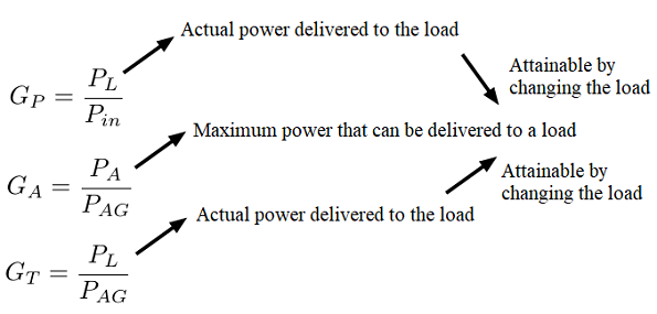
Overview input power within the gains

Comparing and maximizing the power gains

Note: In the next sections, we consider the network Z fixed and change the generator impedance Z_G and/or load impedance Z_L in order to maximize the gains.

Maximizing the operating power gain G_P

The operating power gain G_P is only dependent on the load impedance Z_L and not on the generator impedance Z_G. The question therefore is: "What is the optimal load impedance for maximizing G_P?", or "What is the optimal load for maximizing the efficiency of the system?".

We will call the specific value of the load Z_L that maximizes the operational power gain Z_c2:

G_P= maximum at (Z_L = Z_c2)

The value of Z_c2 can be determined by solving the system of equations [1,2,3]:

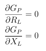
We will later determine the value of Z_c2 by applying another method.

Maximizing the available gain G_A

The available gain G_A is only dependent on the generator impedance Z_G and not on the load impedance Z_L. We will call the specific value of thegenerator impedance Z_G that maximizes the available gain Z_c1:

G_A= maximum at (Z_G = Z_c1)

The value of Z_c2 can be determined by solving the system of equations:

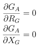
We will later determine the value of Z_c1 by applying another method.

Before maximizing G_T, we will first compare the different gains with each other. It will come clear why we do this, just bear with us...

Comparing the transducer gain G_T to the operating power gain G_P

Since P_in≤ P_AG , it follows that G_T ≤ G_P .

As example, let us consider a very simple, purely resistive network, consisting of three resistors:

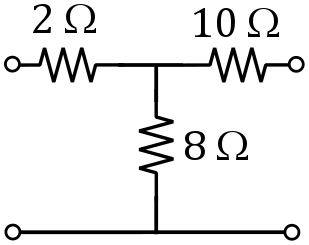
Figure 2: Simple, purely resistive, example network

We simulate the gains in LT Spice with a DC voltage source of 12 V, as function of the generator resistance and the load resistance (details).

We plot G_P (in green) and G_T (in red) as function of varying load resistance (figure 3). The generator impedance was chosen to be 20 ohm. We notice that indeed G_T is always smaller than G_P . A maximum of 10.9% is reached for G_P at a load of 14.5 ohm.

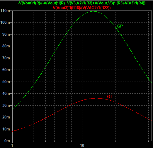
Figure 3: G_P (in green) and G_T (in red) as function of varying load resistance (logarithmic axis) for the example network of figure 2 (details). The generator impedance was chosen to be 20 ohm.

Comparing the transducer gain G_T to the available gain G_A

Since P_L ≤ P_A , it follows that G_T≤ G_A.

For the simple resistive example, we plot G_A (in blue) and G_T (in red) as function of varying generator resistance (figure 4). The load impedance was chosen to be 100 ohm. We notice that indeed G_Tis always smaller than G_A . A maximum of 10.9% is reached for G_P at a load of 8.0 ohm.

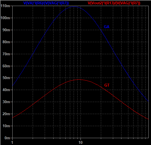
Figure 4: G_A (in blue) and G_T (in red) as function of varying generator resistance (logarithmic axis) for the example network of figure 2 (details). The load impedance was chosen to be 100 ohm.

Comparing the opearational power gain G_P to the available gain G_A

For our example, we plot G_P (in green) as function of varying load resistance, and G_A (in blue) as function of varying generator resistance (figure 5). Notice that both gains have the same maximum of 10.9%.

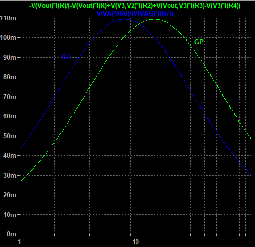
Figure 5: G_P (in green) as function of varying load resistance and G_A (in blue) as function of varying generator resistance (logarithmic axis) for the example network of figure 2 (details).

Maximizing the transducer gain G_T

Taken into account the above, we know that

1. G_T ≤ G_P and G_T≤ G_A
2. G_P is maximum at Z_L = Z_c2 (by definition)
3. G_Ais maximum at Z_G = Z_c1 (by definition)
4. From the definitions of G_T and G_P , we find that G_T = G_P when Z_G = (Z_in)* at the input port. Indeed, in that case, the actual input power P_in equals the maximum attainable input power P_GA (see figure 3 in the previous post).
5. From the definitions of G_T and G_A , we find that G_T = G_A when Z_L = (Z_out)* at the output port. Indeed, in that case, the actual load power P_L equals the maximum maximum available load power P_A (see figure 5 in the previous post).

Combining the five statements above, we find that G_T is maximized if Z_G = (Z_in)* = Z_c1 and Z_L = (Z_out)* = Z_c2

G_T= maximum at Z_G = Z_c1 and Z_L = Z_c2

Notice that under these conditions G_T = G_P = G_A . In other words, if the generator impedance equals (Z_in)* = Z_c1 and the load impedance equals (Z_out)* = Z_c2, the three gains are maximized and equal each other. We will call this value the ultimate gain G_M.

Maximum gains: G_T = G_P = G_A =G_M at Z_G = Z_c1 and Z_L = Z_c2

Indeed, simulating the gains with the optimal generator and load impedance results in the same maximum value for each gain.

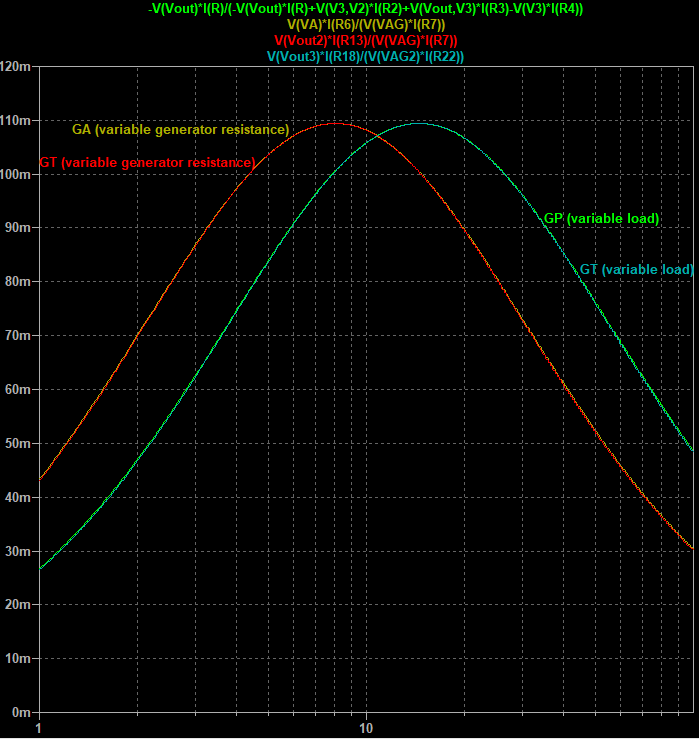
Figure 6: Simulation results of the gains as function of varying generator or load resistance for the given example (details).

Determining Z_c1 and Z_c2

Now that we have found the condition for maximizing the gains, i.e. equalizing the gains to the ultimate gain G_M , we can determine Z_c1 and Z_c2 as function of the network.

The condition we found was (Z_in)* = Z_c1 and (Z_out)* = Z_c2, or

Z_in = (Z_c1)* and Z_out = (Z_c2)* (see figure 7)

Z_c1 and Z_c1 are called the conjugate image impedances.

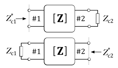
Figure 7: Definition conjugate image impedances

If we consider the network Z to be a two-port network characterized by its impedance matrix Z with 2x2 matrix elements z_ij=r_ij+jx_ij (i,j = 1,2), the input and output impedance equals:

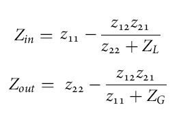
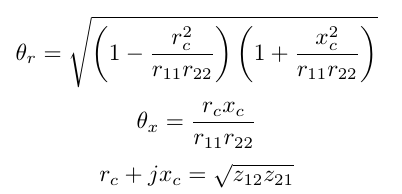
Solving the system (Z_in)* = Z_c1 and (Z_out)* = Z_c2 for Z_G= Z_c1 and Z_L= Z₂ results in the conjugate image impedances Z_c1=R_c1+jX_c1 and Z_c2=R_c2+jX_c2 that maximize the gains [1,4,5,6]:

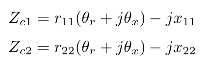
with

For the simulation example of 2 (z₁₁=10, z₁₂= z₂₁=8, z₂₂=18), we find Z_c1= 8.0 ohm and Z_c1= 14.5 ohm, corresponding to the simulation results.

 

References

[1] Ben Minnaert and Nobby Stevens. Single variable expressions for the efficiency of a reciprocal power transfer system. International Journal of Circuit Theory and Applications, 45 (10), (2017). 1418-1430.
Paper: [pdf]

[2] Dionigi M, Mongiardo M, Perfetti R. Rigorous network and full-wave electromagnetic modeling of wireless power transfer links. IEEE
Transactions on Microwave Theory and Techniques 2015; 63(1), pp. 65-75, DOI: 10.1109/TMTT.2014.2376555.

[3] Bird TS, Rypkema N, Smart KW. Antenna impedance matching for maximum power transfer in wireless sensor networks. IEEE Sensors
2009; pp. 916-919, DOI: 10.1109/ICSENS.2009.5398165.

[4] Roberts, S. (1946). Conjugate-image impedances. Proceedings of the IRE, 34(4), 198p-204p.

[5] Mastri, F., Mongiardo, M., Monti, G., Dionigi, M., & Tarricone, L. (2018). Gain expressions for resonant inductive wireless power transfer links with one relay element. Wireless Power Transfer, 5(1), 27-41.

[6] Ben Minnaert, Giuseppina Monti, Alessandra Costanzo and Mauro Mongiardo, Gain Expressions for Capacitive Wireless Power Transfer with One Electric Field Repeater. Electronics 2021, 10, 723.
Paper: [pdf]