About - Publications - Blog

Different Power Gains

Types of power gain

If you hear the word 'power gain', you justly interpret this as the ratio of the output power P_out to the input power P_in:

Unfortunately, confusion is possible, since there are different ways to define the ouput and input power. And depending on which definition of power you use, you get another value for the gain. But mankind has found a solution: we use different names for the gains, depending on which power is considered. Let us try to give an overview of the three most common gains.

A two-port network, connected to a source and a load.

Consider a network "Z" with one input and one output (a two-port network). The input is connected to a generator (a voltage source V_G with internal impedance Z_G=R_G+j.X_G) and the output to a load impedance Z_L=R_L+j.X_L.

• We call the input impedance of the network Z_in=R_in+j.X_in. Note that the input impedance Z_in is dependent on Z_L (see figure 1).
• We call the output impedance Z_out=R_out+j.X_out. Note that the output impedance Z_inis dependent on Z_G (see figure 1).

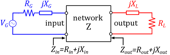
Figure 1: A network Z is connected to a generator at the input, and a load at the output

We will define three different types of gain for the network Z. We first start by considering two different definitions of input power.

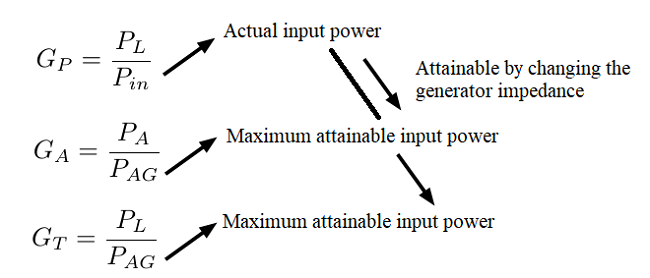
Different types of input power

Actual input power P_in

The actual input power P_in (usually simply called 'the input power') is the power that the generator delivers to the network Z, connected to a load Z_L. It is the power dissipated in R_inas seen in the following figure.

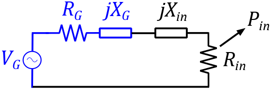
Figure 2: Definition actual input power

As a result, the input power is dependent not only on the network Z, but also on the value of Z_L. It is independent on Z_G.

This implies that a load impedance Z_Lmust be explicitely specified in order to be able to define the actual input power P_in.

Available input power P_AG

The available input power P_AG (often called 'the available input power of the generator') is the maximum input power that can be put into the network Z by a generator. This is achieved for a specific value of the load, i.e., if the load value is chosen so that the input impedance Z_in of the network is matched (= equal resistance, opposite reactance) to the generator impedance Z_G.

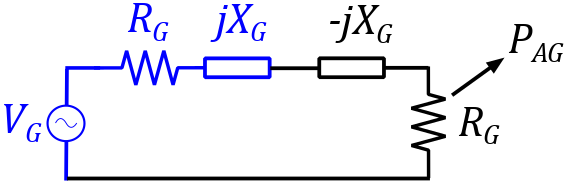
Figure 3: Definition available input power

The available input power for the network is only dependent on the value of Z_G. It is independent on the network Z or Z_L since both are together matched to the generator impedance.

This implies that the generator impedance must be specified in order to be able to define the available input power.

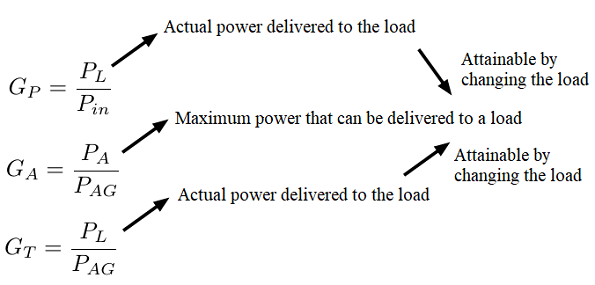
Different types of output power

The power delivered to the load P_L

It is the power dissipated in the load Z_Las seen in the following figure.

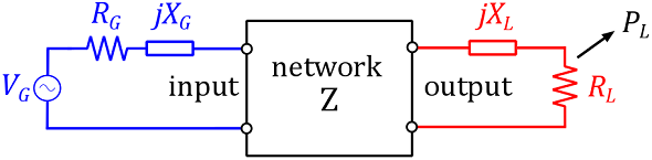
Figure 4: Definition power delivered to the load

Note that P_L is dependent on the value of the load and not on the generator impedance. This implies that a load impedance Z_Lmust be explicitely specified in order to be able to define P_L.

The maximum available load power P_A

The maximum available load power P_A is the maximum power that can be dissipated into the load. This is realized for a specific value of the load, i.e., if the load value is chosen so that the output impedance Z_out of the network is matched (= equal resistance, opposite reactance) to the load impedance Z_L. In other words, the maximum available load power is the power the network delivers to a load that is matched to its output impedance.

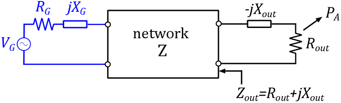
Figure 5: Definition maximum available load power

The maximum available load power P_A for the network is dependent on the value of Z_G and the network Z. It is independent on the load Z_L.

This implies that the generator impedance must be specified in order to be able to define P_A.

Three different power gains

It is now possible to define different power gains, depending on which definittion of input and output power is chosen. We will limit ourselve to the three most common power gains.

The operating power gain G_P

The operating power gain G_P (often simply called 'the power gain' or 'actual gain') is defined as the ratio of the power dissipated in the load Z_L to the power that the generator delivers to the network Z, connected to that load Z_L:

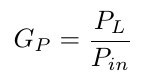
Since both P_L and P_in are independent on the generator impedance Z_G, the operating power gain G_P is also independent on Z_G. The generator impedance does not need to be specified: we just need to know how much power got to the network, not how it got there.

The gain depends on the network Z and on the load value Z_L. Obviously, G_P can only be defined if a value for the load Z_L is specified.

In systems where the goal is to transfer energy from a source to a load, the operating power gain is often called 'the power conversion efficiency', or simply 'the efficiency" of the system.

Available gain G_A

The available gain G_A is defined as the ratio of the maximum available load power P_A to the available input power P_AG :

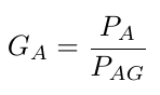
Since both P_A and P_AG are independent on the load impedance Z_L, the available gain G_A is also independent on Z_L. The gain depends on the network Z and on the generator impedance value Z_G.

Obviously, G_A can only be defined if a value for the generator impedance Z_G is specified.

Transducer gain G_T

The transducer gain G_T is defined as the ratio of the power dissipated in the load Z_L to the available input power P_AG of the generator:

It is dependent on both the load impedance Z_L and the generator impedance Z_G. Both have to be specified in order to be able to define the transducer gain G_T.

Overview output power within the gains

Overview input power within the gains

Simulation example

As example, let us consider a very simple, purely resistive network, consisting of three resistors:

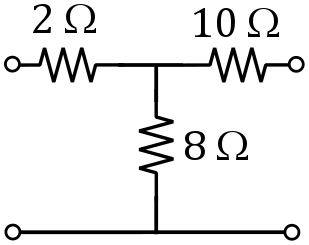
Figure 6: Simple, purely resistive, example network

We simulate the three gains in LT Spice with a DC voltage source of 12 V, as function of the generator resistance and the load resistance.

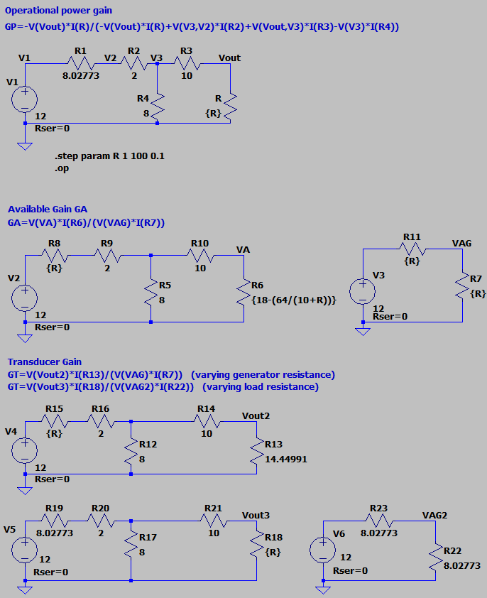
Figure 7: Schematics in LT Spice for the three gains, for the example network, with variable load and/or generator resistance {R}.

We first simulate the operating power gain G_P as function of the load resistance. This gain is independent on the generator resistance. In the simulation, a generator resistance of 8.02773 ohm was chosen (see further), but this value doesn't matter for the simulation of the operating power gain G_P.

The graph below (green) shows that a maximum of G_P = 10.9% is reached for a load of 14.5 ohm.

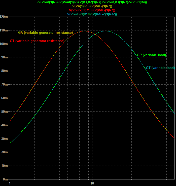
Figure 8: Simulation results of the gains as function of varying generator or load resistance (logaritmic axis) for the given example.

Next, the available gain G_A is simulated as function of varying generator resistance (this gains is independent on the value of the load). We find a maximum of 10.9% at a generator resistance of 8.0 ohm.

Finally, the transducer gain G_T is simulated, first for varying generator resistance, and next for varying load. The genenerator/load resistance in each non-varying case is chosen to be the optimal value for the other gains. The graphs are identical to the other gains (explanation). A maximum of 10.9% is found for the optimal generator and load resistance of 8.0 and 14.5 ohm.

Some background references

• Egan,W.F. Practical RF System Design; JohnWiley & Sons: Hoboken, NJ, USA, 2003; pp. 313–315.
• Mastri, F.; Mongiardo, M.; Monti, G.; Dionigi, M.; Tarricone, L. Gain Expressions for Resonant Inductive Wireless Power Transfer
  Links with One Relay Element. Wireless Power Transfer 2018, 5, 27–41.
• Ben Minnaert, Giuseppina Monti, Alessandra Costanzo and Mauro Mongiardo, Gain Expressions for Capacitive Wireless Power Transfer with One Electric Field Repeater. Electronics 2021, 10, 723.
  Paper: [pdf]